Budget Allocation with PyMC-Marketing

The purpose of this notebook is to explore the recently included function in the PyMC-Marketing library that focuses on budget allocation. This function’s underpinnings are based on the methodologies inspired by Bolt’s work in the article, “Budgeting with Bayesian Models”.

Prerequisite Knowledge

The notebook assumes the reader has knowledge of the essential functionalities of PyMC-Marketing. If one is unfamiliar, the “MMM Example Notebook” serves as an excellent starting point, offering a comprehensive introduction to media mix models in this context.

Introducing the budget allocator

This notebook instigates an examination of the function within the PyMC-Marketing library, which addresses these challenges using Bayesian models. The function intends to provide:

1. Quantitative measures of the effectiveness of different media channels.

2. Probabilistic ROI estimates under a range of budget scenarios.

Basic Setup

Like previous notebooks revolving around PyMC-Marketing, this relies on a specific library set. Here are the requisite imports necessary for executing the provided code snippets subsequently.

import warnings

import arviz as az
import matplotlib.pyplot as plt
import numpy as np
import pandas as pd
import xarray as xr

from pymc_marketing.mmm.builders.yaml import build_mmm_from_yaml
from pymc_marketing.mmm.multidimensional import (
    MultiDimensionalBudgetOptimizerWrapper,
)
from pymc_marketing.paths import data_dir

warnings.filterwarnings("ignore")

az.style.use("arviz-darkgrid")
plt.rcParams["figure.figsize"] = [12, 7]
plt.rcParams["figure.dpi"] = 100

%load_ext autoreload
%autoreload 2
%config InlineBackend.figure_format = "retina"

OMP: Info #276: omp_set_nested routine deprecated, please use omp_set_max_active_levels instead.
/Users/carlostrujillo/Documents/GitHub/pymc-marketing/pymc_marketing/mmm/multidimensional.py:72: FutureWarning: This functionality is experimental and subject to change. If you encounter any issues or have suggestions, please raise them at: https://github.com/pymc-labs/pymc-marketing/issues/new
  warnings.warn(warning_msg, FutureWarning, stacklevel=1)
/var/folders/f0/rbz8xs8s17n3k3f_ccp31bvh0000gn/T/ipykernel_38045/3141621575.py:9: UserWarning: The pymc_marketing.mmm.builders module is experimental and its API may change without warning.
  from pymc_marketing.mmm.builders.yaml import build_mmm_from_yaml

These imports and configurations form the fundamental setup necessary for the entire span of this notebook.

The expectation is that a model has already been trained using the functionalities provided in prior versions of the PyMC-Marketing library. Thus, the data generation and training processes will be replicated in a different notebook. Those unfamiliar with these procedures are advised to refer to the “MMM Example Notebook.”

Loading a Pre-Trained Model

To utilize a saved model, load it into a new instance of the MMM class using the build_mmm_from_yaml method below.

seed: int = sum(map(ord, "mmm_allocation_example"))
rng: np.random.Generator = np.random.default_rng(seed=seed)

data_path = data_dir / "multidimensional_mock_data.csv"
data_df = pd.read_csv(data_path, parse_dates=["date"], index_col=0)
data_df.head()

	date	y	x1	x2	event_1	event_2	dayofyear	t	geo
0	2018-04-02	3984.662237	159.290009	0.0	0.0	0.0	92	0	geo_a
1	2018-04-09	3762.871794	56.194238	0.0	0.0	0.0	99	1	geo_a
2	2018-04-16	4466.967388	146.200133	0.0	0.0	0.0	106	2	geo_a
3	2018-04-23	3864.219373	35.699276	0.0	0.0	0.0	113	3	geo_a
4	2018-04-30	4441.625278	193.372577	0.0	0.0	0.0	120	4	geo_a

x_train = data_df.drop(columns=["y"])
y_train = data_df["y"]

mmm = build_mmm_from_yaml(
    X=x_train,
    y=y_train,
    config_path=data_dir / "config_files" / "multi_dimensional_example_model.yml",
)

For more details on the build_mmm_from_yaml, consult the pymc-marketing documentation on Model Deployment.

Alternatively, load a model that has been saved to MLflow via pymc_marketing.mlflow.log_inference_data or has been autologged to MLflow via pymc_marketing.mlflow.autolog(log_mmm=True), from the PyMC-Marketing MLflow module.

## If you have a hosted MLflow server, you will of course need to authenticate first.
# RUN_ID = "your_run_id"
# from pymc_marketing.mlflow import load_mmm
# mmm = load_mmm(RUN_ID)

# # Load the full model with the InferenceData
# mmm = load_mmm(
#     run_id=RUN_ID,         # The MLflow run ID from which to load the model
#     full_model=True,       # Set to True to get the full MMM model with InferenceData
#     keep_idata=True,       # Set to True if you want to keep the downloaded InferenceData saved locally
# )

Problem Statement

Before jumping into the data, let’s first define the business problem we are trying to solve. In a progressively competitive scenario, marketers are tasked with distributing a predetermined marketing budget across various channels to maximize a certain response. Consider a forthcoming quarter wherein a marketing team must decide the division of its operations between two advertising channels, represented as x1 and x2. These could effectively symbolize any medium, such as TV, digital advertising, print, etc.

The task lies in making decisions that invoke data, comply with factual evidence, and align with business logic. For instance, how can one incorporate prior information like budget restrictions, platform trends, constraints, or even distinctive features of each channel into the decision-making process?

Introducing Budget Allocation Function

The budget allocation capabilities in PyMC-Marketing aims to tackle this issue by offering a Bayesian framework for optimal allocation. This enables marketers to:

• Integrate the outcomes of Media Mix Modeling (MMM), quantifying each channel’s effectiveness in metrics like ROI, incremental sales, etc.

• Merge this empirical data with prior business knowledge and logic for making holistic and robust decisions.

By utilizing this function, marketers can guarantee that the budget spread not only obeys the mathematical rigor furnished by the MMM outcomes but also incorporates business-specific factors, thereby achieving a balanced and optimized budget plan.

Getting started

Media Mix Modeling (MMM) acts as a dependable method to estimate the contribution of each channel (e.g., x1, x2) to a target variable like sales or any variable.

The function saturation_scatterplot() allows for visualization of this direct channel impact. However, it is crucial to remember that this only unveils the “observable space” for values of X (spend) and Y (contribution).

mmm.plot.saturation_scatterplot(original_scale=True);

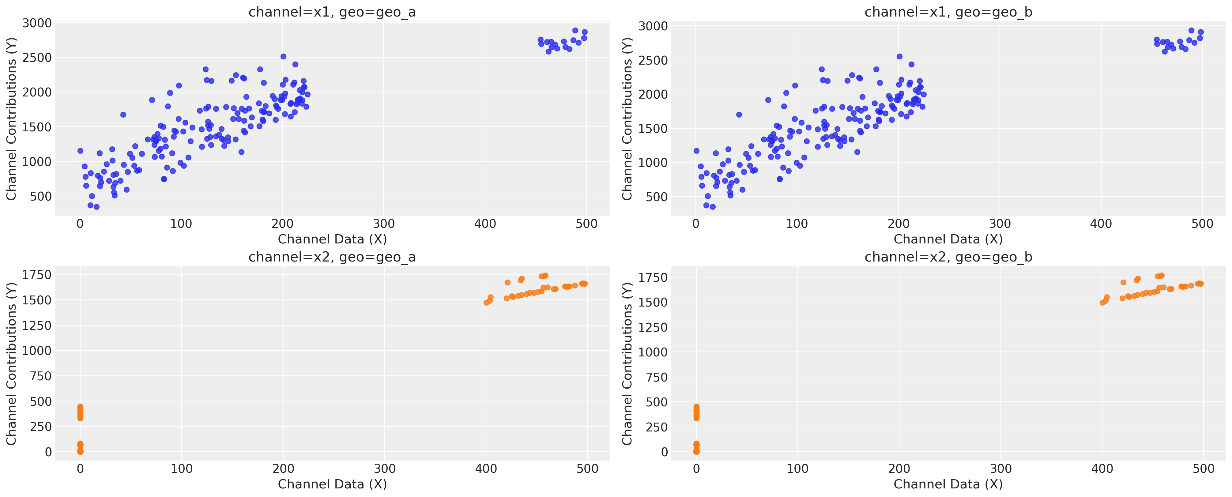
The observable space only encompasses our data points and does not illustrate what transpires beyond those points. As a result, it is not assured that the maximum contribution point for each channel lies within this observable range.

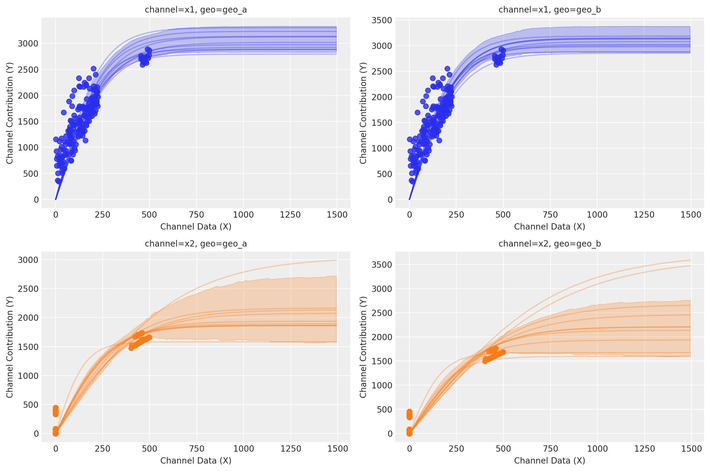
If we want to visualize certain level of response, we can use sample_curve to get an estimate of our response in scaled space given a max value of X in scaled space as well. In the example below, we are using the value 3 which represent 3X the max historical value on each channel. Depending on your scaling method, max_value could represent a different thing.

After it, using the function saturation_curves, we can predict the shape of the model fitting curve for the amount spent that was not previously observed.

curve = mmm.saturation.sample_curve(
    mmm.idata.posterior[["saturation_beta", "saturation_lam"]], max_value=3
)
fig, axes = mmm.plot.saturation_curves(
    curve,
    original_scale=True,
    n_samples=10,
    hdi_probs=0.85,
    random_seed=rng,
    subplot_kwargs={"figsize": (12, 8), "ncols": 2},
    rc_params={
        "xtick.labelsize": 10,
        "ytick.labelsize": 10,
        "axes.labelsize": 10,
        "axes.titlesize": 10,
    },
)

for ax in axes.ravel():
    ax.title.set_fontsize(10)

if fig._suptitle is not None:
    fig._suptitle.set_fontsize(12)

plt.tight_layout()
plt.show()

Sampling: []

We can identify which saturation function was used in the pre-trained model:

print(f"Model was train using the {mmm.saturation.__class__.__name__} function")
print(f"and the {mmm.adstock.__class__.__name__} function")

Model was train using the LogisticSaturation function
and the GeometricAdstock function

Within PyMC-Marketing we have different saturation functions, you can observe all in the transformer module.

Once these parameters are obtained, you can visualize it using the arviz.summary function (each parameter has the prefix saturation or adstock respectively) and, if desired, you can recreate the curves for each channel independently based on them. More crucially, these parameter values are indispensable when using the budget_allocator function, which leverages this information to optimize your marketing budget across distinct channels. This section is fundamental to budget optimization.

az.summary(
    data=mmm.fit_result,
    var_names=[
        "saturation_beta",
        "saturation_lam",
        "adstock_alpha",
    ],
)

	mean	sd	hdi_3%	hdi_97%	mcse_mean	mcse_sd	ess_bulk	ess_tail	r_hat
saturation_beta[x1]	0.370	0.021	0.332	0.409	0.001	0.001	565.0	537.0	1.01
saturation_beta[x2]	0.269	0.061	0.182	0.384	0.003	0.003	552.0	499.0	1.01
saturation_lam[x1]	4.025	0.409	3.242	4.756	0.016	0.013	625.0	490.0	1.00
saturation_lam[x2]	2.815	1.091	1.139	4.744	0.053	0.060	492.0	430.0	1.01
adstock_alpha[x1]	0.395	0.032	0.331	0.453	0.001	0.001	728.0	555.0	1.00
adstock_alpha[x2]	0.178	0.043	0.104	0.266	0.002	0.001	624.0	325.0	1.01

Example Use-Cases

The optimize_budget function within PyMC-Marketing boasts a myriad of applications that can solve various business predicaments. Here, we present five critical use cases that exemplify its utility in real-world marketing scenarios.

What are we optimizing?

Before jumping into the examples, we need to understand the basis of our optimizer.

We aim to optimize the allocation of budgets across multiple channels to maximize the overall contribution to key performance indicators (KPIs), such as sales or conversions. Each channel has its own forward pass function, which can internal consider a sigmoid or michaelis-menten curve, representing the relationship between the amount spent and the resultant performance.

These curves vary in characteristics: some channels saturate quickly, meaning that additional spending yields diminishing returns, while others may offer more linear growth in contribution with increased spending.

To solve this optimization problem, we employ the Sequential Least Squares Quadratic Programming (SLSQP) algorithm, a gradient-based optimization technique. SLSQP is well-suited for this application as it allows for the imposition of both equality and inequality constraints, ensuring that the budget allocation adheres to business rules or limitations.

The algorithm works by iteratively approximating the objective function and constraints using quadratic functions and solving the resulting sub-problems to find a local minimum. This enables us to effectively navigate the multidimensional space of budget allocations to find the most efficient distribution of resources.

The optimizer aims to maximize the total contribution from all channels while adhering to the following constraints:

1. Budget Limitations: The total spending across all channels should not exceed the overall marketing budget.

2. Channel-specific Constraints: Some channels may have minimum or maximum spending limits.

By leveraging the SLSQP algorithm, we can optimize the multi-channel budget allocation in a rigorous, mathematically sound manner, ensuring that we get the highest possible return on investment.

Maximizing Contribution

Assume you’re managing the marketing for a retail company with a substantial budget to allocate for advertising across multiple channels. Given that, you’re contemplating ways to optimize the forthcoming quarter’s outlay to maximize the overall contribution.

You might have considered scattering your money in the same way than you did historically without an MMM model - let’s repeat the know formula. However, you wish to explore better alternatives now that you possess an MMM model. Given that you lack prior knowledge, you impose the same restrictions on both channels. They must each expend a minimum of 500 euros and no more than 2,000 euros, equating to your total budget.

from pymc_marketing.mmm.budget_optimizer import optimizer_xarray_builder

time_unit_budget = 4_000  # Budget per time unit
campaign_period = 12  # Number of time units
print(
    f"Total budget for the {campaign_period} Weeks: {time_unit_budget * campaign_period:,}"
)
# Define your channels
channels = ["x1", "x2"]
geos = ["geo_a", "geo_b"]
# The initial split per channel
budget_per_channel = time_unit_budget / (len(channels) * len(geos))
# Initial budget per channel.
initial_budget = optimizer_xarray_builder(
    np.array(
        [
            [budget_per_channel * 0.5, budget_per_channel * 1.5],
            [budget_per_channel * 0.6, budget_per_channel * 1.4],
        ]
    ),
    channel=channels,
    geo=geos,
)  # Using this function we can create the initial allocation strategy for each channel and geo

print("-" * 50)
print("Budget per channel per geo:")
for geo in geos:
    for channel in channels:
        print(
            f"  {geo} - {channel}: {initial_budget.sel(geo=geo, channel=channel).item():.2f}"
        )

# bounds for each channel
min_budget, max_budget = 500, 2_000
budget_bounds = optimizer_xarray_builder(
    np.array(
        [
            [[min_budget, max_budget], [min_budget, max_budget]],
            [[min_budget, max_budget], [min_budget, max_budget]],
        ]
    ),
    channel=channels,
    geo=geos,
    bound=["lower", "upper"],
)  # Using this function we can create a budget bounds for each channel and geo as well

Total budget for the 12 Weeks: 48,000
--------------------------------------------------
Budget per channel per geo:
  geo_a - x1: 500.00
  geo_a - x2: 600.00
  geo_b - x1: 1500.00
  geo_b - x2: 1400.00

Our current model was trained with weekly data, meaning each period (time unit) represents a week. If we plan to create a budget allocation for a specific quarter, we need to add 12 weeks to our initial date. By doing so, we can initialize our class that wraps our MMM.

# Get the maximum date and add one day to it
max_date = mmm.idata.posterior.coords["date"].max().item()
start_date = (
    pd.Timestamp(max_date) + pd.Timedelta(weeks=1)
).strftime(  # mmm.adstock.l_max+2
    "%Y-%m-%d"
)

end_date = (pd.Timestamp(start_date) + pd.Timedelta(weeks=campaign_period)).strftime(
    "%Y-%m-%d"
)

print(f"Start date: {start_date}, End date: {end_date}")

Start date: 2021-09-06, End date: 2021-11-29

optimizable_model = MultiDimensionalBudgetOptimizerWrapper(
    model=mmm, start_date=start_date, end_date=end_date
)

optimizable_model.adstock.l_max, optimizable_model.num_periods

Before we proceed to evaluate the effectiveness of our optimization, we can estimate the response by following our initial plan, which involves distributing our budget based on historical spending patterns.

sample_response_give_initial_budget = optimizable_model.sample_response_distribution(
    allocation_strategy=initial_budget,  # Here we add the initial budget allocation strategy
    include_carryover=True,
    include_last_observations=False,
)

Sampling: [y]

The response will be expose as a data array with different variables, such as:

• y (Target variables)

• allocation (The allocation strategy shared)

• channel variables (Every channel column with the corresponding units used to get the prediction).

• Total Media Channel Contribution in Original Scale (The posterior distribution of the sum of media channel by date)

initial_budget.sum(dim="geo")

<xarray.DataArray (channel: 2)> Size: 16B
array([2000., 2000.])
Coordinates:
  * channel  (channel) <U2 16B 'x1' 'x2'

xarray.DataArray

• channel: 2

• 2e+03 2e+03

  array([2000., 2000.])

• Coordinates: (1)
  • channel
    (channel)
    <U2
    'x1' 'x2'

    array(['x1', 'x2'], dtype='<U2')

• Indexes: (1)
  • channel
    PandasIndex

    PandasIndex(Index(['x1', 'x2'], dtype='object', name='channel'))

• Attributes: (0)

sample_response_give_initial_budget.allocation.sum(dim="geo")

<xarray.DataArray 'allocation' (channel: 2)> Size: 16B
array([2000., 2000.])
Coordinates:
  * channel  (channel) <U2 16B 'x1' 'x2'

xarray.DataArray

'allocation'

• channel: 2

• 2e+03 2e+03

  array([2000., 2000.])

• Coordinates: (1)
  • channel
    (channel)
    <U2
    'x1' 'x2'

    array(['x1', 'x2'], dtype='<U2')

• Indexes: (1)
  • channel
    PandasIndex

    PandasIndex(Index(['x1', 'x2'], dtype='object', name='channel'))

• Attributes: (0)

sample_response_give_initial_budget["x1"].sum(dim="geo")

<xarray.DataArray 'x1' (date: 21)> Size: 168B
array([2001.05516828, 1998.17680521, 2000.86259682, 2000.53354004,
       2001.24720109, 2001.03767898, 2000.10398136, 2002.55438021,
       2000.10373669, 1999.06157133, 2000.07774446, 2000.98811459,
       2000.96803296,    0.        ,    0.        ,    0.        ,
          0.        ,    0.        ,    0.        ,    0.        ,
          0.        ])
Coordinates:
  * date     (date) datetime64[ns] 168B 2021-09-06 2021-09-13 ... 2022-01-24

xarray.DataArray

'x1'

• date: 21

• 2.001e+03 1.998e+03 2.001e+03 2.001e+03 2.001e+03 ... 0.0 0.0 0.0 0.0

  array([2001.05516828, 1998.17680521, 2000.86259682, 2000.53354004,
         2001.24720109, 2001.03767898, 2000.10398136, 2002.55438021,
         2000.10373669, 1999.06157133, 2000.07774446, 2000.98811459,
         2000.96803296,    0.        ,    0.        ,    0.        ,
            0.        ,    0.        ,    0.        ,    0.        ,
            0.        ])

• Coordinates: (1)
  • date
    (date)
    datetime64[ns]
    2021-09-06 ... 2022-01-24

    array(['2021-09-06T00:00:00.000000000', '2021-09-13T00:00:00.000000000',
           '2021-09-20T00:00:00.000000000', '2021-09-27T00:00:00.000000000',
           '2021-10-04T00:00:00.000000000', '2021-10-11T00:00:00.000000000',
           '2021-10-18T00:00:00.000000000', '2021-10-25T00:00:00.000000000',
           '2021-11-01T00:00:00.000000000', '2021-11-08T00:00:00.000000000',
           '2021-11-15T00:00:00.000000000', '2021-11-22T00:00:00.000000000',
           '2021-11-29T00:00:00.000000000', '2021-12-06T00:00:00.000000000',
           '2021-12-13T00:00:00.000000000', '2021-12-20T00:00:00.000000000',
           '2021-12-27T00:00:00.000000000', '2022-01-03T00:00:00.000000000',
           '2022-01-10T00:00:00.000000000', '2022-01-17T00:00:00.000000000',
           '2022-01-24T00:00:00.000000000'], dtype='datetime64[ns]')

• Indexes: (1)
  • date
    PandasIndex

    PandasIndex(DatetimeIndex(['2021-09-06', '2021-09-13', '2021-09-20', '2021-09-27',
                   '2021-10-04', '2021-10-11', '2021-10-18', '2021-10-25',
                   '2021-11-01', '2021-11-08', '2021-11-15', '2021-11-22',
                   '2021-11-29', '2021-12-06', '2021-12-13', '2021-12-20',
                   '2021-12-27', '2022-01-03', '2022-01-10', '2022-01-17',
                   '2022-01-24'],
                  dtype='datetime64[ns]', name='date', freq=None))

• Attributes: (0)

fig, ax = plt.subplots()
az.plot_posterior(
    sample_response_give_initial_budget.total_media_contribution_original_scale.values.flatten(),
    hdi_prob=0.95,
    color="blue",
    label="Intial planned allocation",
    ax=ax,
);

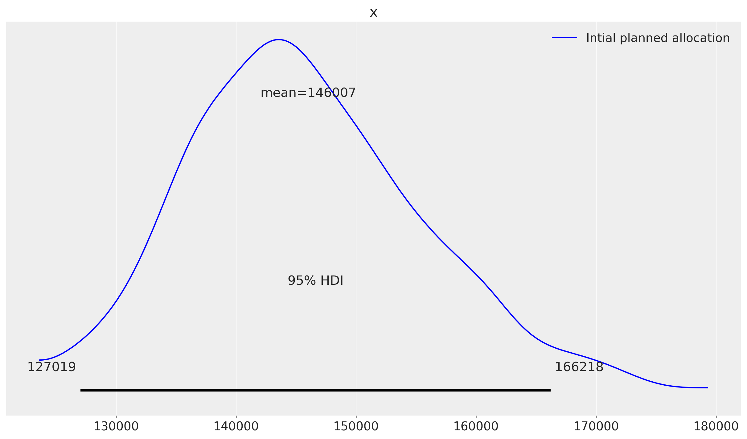
Great, we can see that our initial estimation it’s giving us around 146K new units (sales in this case) given marketing. But given the same budget, could we do better?

allocation_xarray, res_scipy = optimizable_model.optimize_budget(
    budget=time_unit_budget,  # Total budget to allocate here is spend in Millions
    budget_bounds=budget_bounds,  # Budget bounds for each channel
)

sample_response_given_allocation = optimizable_model.sample_response_distribution(
    allocation_strategy=allocation_xarray,
    include_carryover=True,
    include_last_observations=False,
)

Sampling: [y]

res_scipy

     message: Optimization terminated successfully
     success: True
      status: 0
         fun: -150857.9378371236
           x: [ 9.660e+02  1.027e+03  9.745e+02  1.033e+03]
         nit: 22
         jac: [-4.029e+00 -4.029e+00 -4.029e+00 -4.029e+00]
        nfev: 22
        njev: 22
 multipliers: [-4.029e+00]

fig, ax = plt.subplots()

# Initial planned allocation
initial_data = sample_response_give_initial_budget.total_media_contribution_original_scale.values.flatten()
initial_mean = initial_data.mean()
az.plot_dist(
    initial_data,
    # hdi_prob=0.75,
    color="blue",
    label=f"Intial planned allocation: Response {initial_mean:,.0f}",
    ax=ax,
    # kind="hist",
)
ax.axvline(initial_mean, color="blue", linestyle="--")

# Optimized allocation
optimized_data = sample_response_given_allocation.total_media_contribution_original_scale.values.flatten()
optimized_mean = optimized_data.mean()
az.plot_dist(
    optimized_data,
    # hdi_prob=0.75,
    color="red",
    label=f"Optimized allocation: Response {optimized_mean:,.0f}",
    ax=ax,
    # kind="hist",
)
ax.axvline(optimized_mean, color="red", linestyle="--")

ax.set_title("Comparison of Intial and Optimized allocation")
ax.set_xlabel("Response")
ax.set_ylabel("Density")
ax.legend()

plt.show()

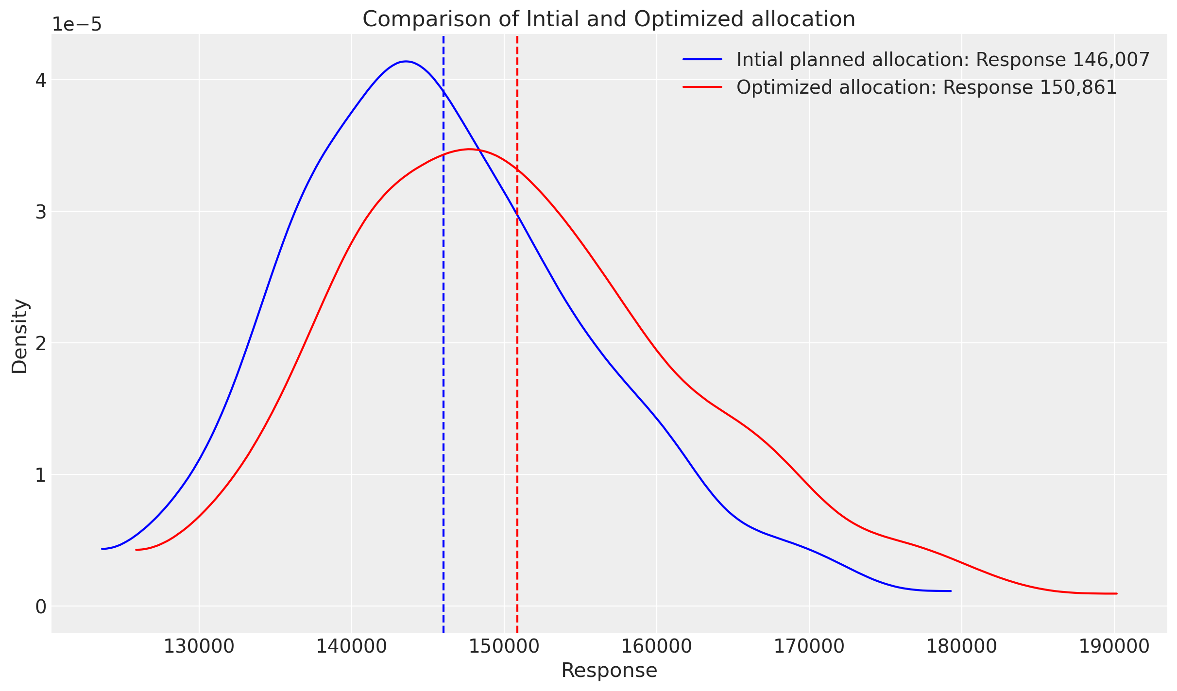
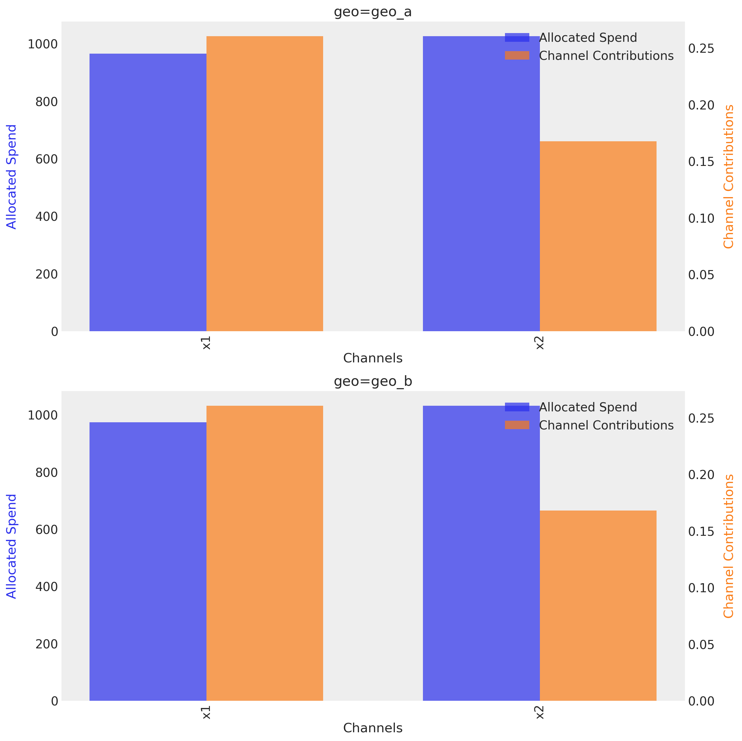
Great, we can see that given the allocation the optimizer maximize the total response from both channel, and give us back 5,000 extra units, given the same spend. We can visualize the mean response per channel, given the spend using the function plot.budget_allocation

optimizable_model.plot.budget_allocation(
    samples=sample_response_given_allocation,
);

We could visualize the response over time if we want.

optimizable_model.plot.allocated_contribution_by_channel_over_time(
    samples=sample_response_given_allocation,
);

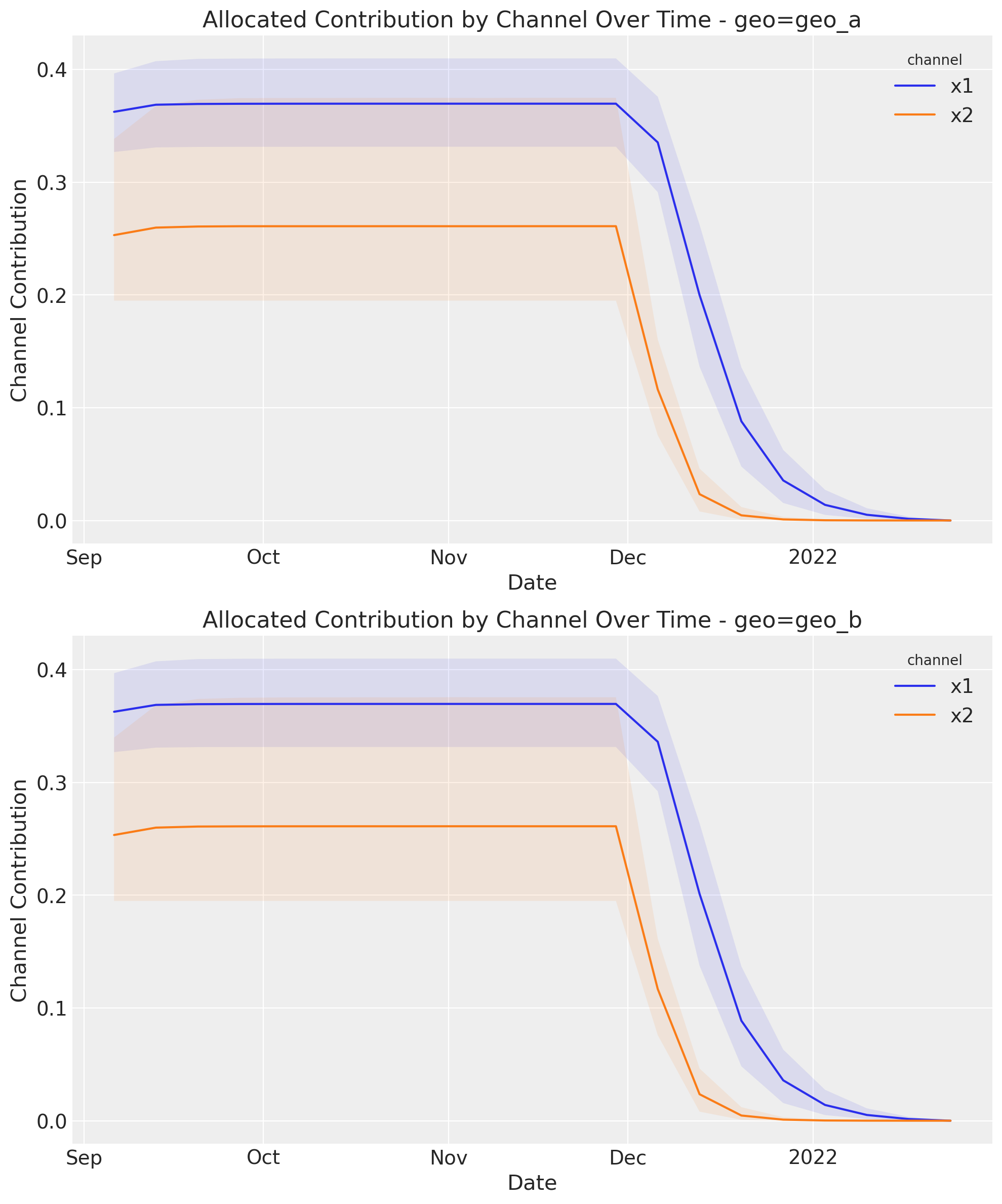
As you probably observe, the response it’s quite flat and saturated. As shown before in the joint distribution of the sum of effects, the mean only increase because the uncertanty was bigger, but majority of the density it’s not to far from the biggest density in the initial allocation.

Why this happens? let’s take a look to the response curves!

curve = mmm.saturation.sample_curve(
    mmm.idata.posterior[["saturation_beta", "saturation_lam"]], max_value=3
)
fig, axes = mmm.plot.saturation_curves(
    curve,
    original_scale=True,
    n_samples=10,
    hdi_probs=0.85,
    random_seed=rng,
    subplot_kwargs={"figsize": (12, 8), "ncols": 2},
    rc_params={
        "xtick.labelsize": 10,
        "ytick.labelsize": 10,
        "axes.labelsize": 10,
        "axes.titlesize": 10,
    },
)

# Add vertical lines for each geo-channel combo from the allocation
channels = sample_response_given_allocation.channel.values
geos = sample_response_given_allocation.geo.values

# Iterate over all channel-geo combinations
subplot_idx = 0
for channel in channels:
    for geo in geos:
        # Make sure we're accessing the correct axis object
        ax = axes.flat[subplot_idx] if isinstance(axes, np.ndarray) else axes

        # Get the budget value for this specific channel-geo combination
        budget_value = sample_response_given_allocation.allocation.sel(
            channel=channel, geo=geo
        ).item()

        # Add vertical line with a label
        ax.axvline(
            x=budget_value,
            color="red",
            linestyle="--",
            label=f"{channel}-{geo}: {budget_value:.1f}",
        )

        subplot_idx += 1

# Ensure we're working with actual axes objects, not numpy arrays
for i in range(len(channels) * len(geos)):
    ax = axes.flat[i] if isinstance(axes, np.ndarray) else axes
    if hasattr(ax, "title"):
        ax.title.set_fontsize(10)

if hasattr(fig, "_suptitle") and fig._suptitle is not None:
    fig._suptitle.set_fontsize(12)

plt.tight_layout()
plt.show()

Sampling: []

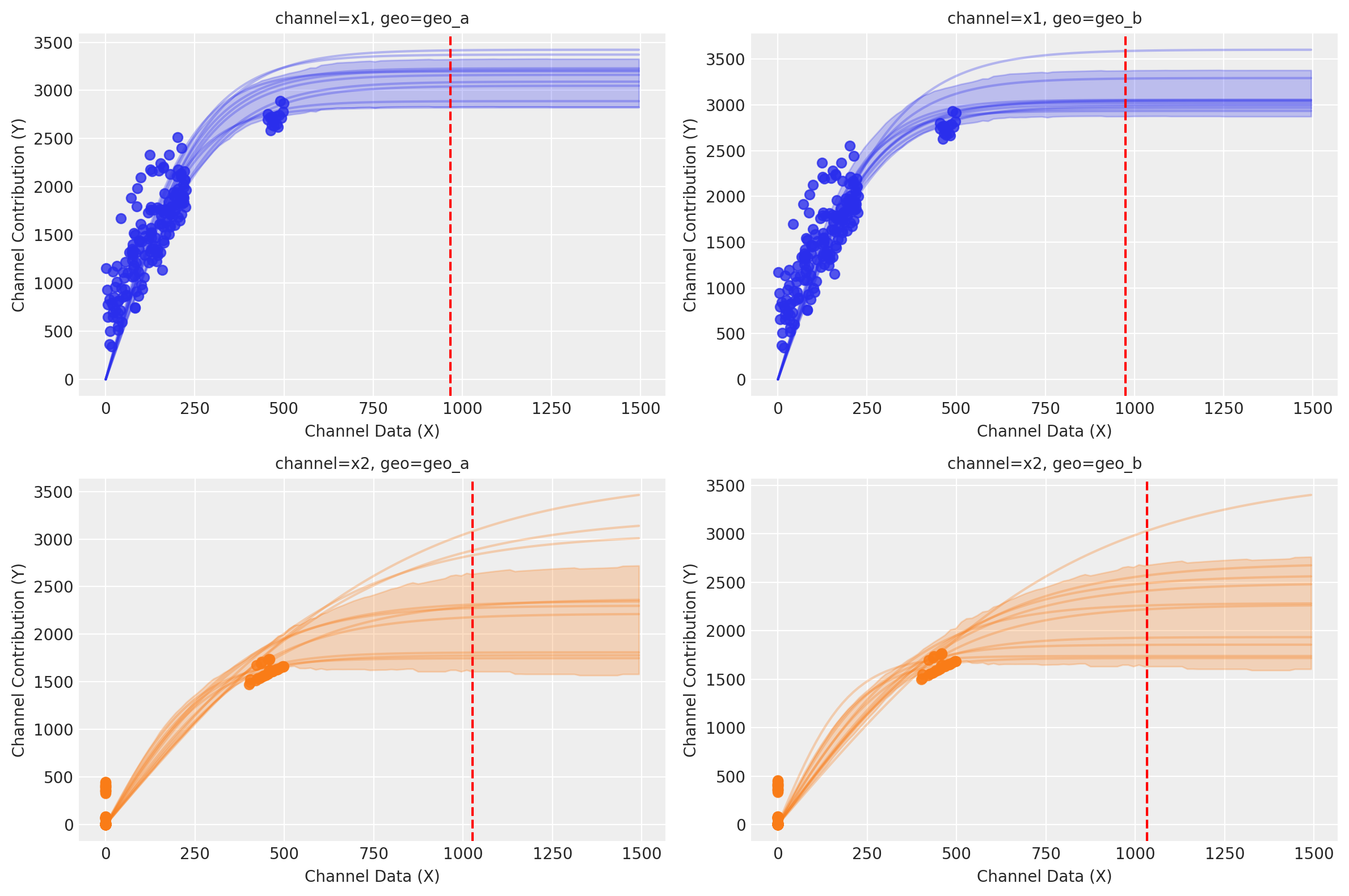
As expected, the allocated budget (red line) lies into the saturation zone, meaning, we have very little movement given the current spend. At least for some channels.

We can iterate over different budgets, adding a bit less or more and validate how much our response move forward given the additional budget.

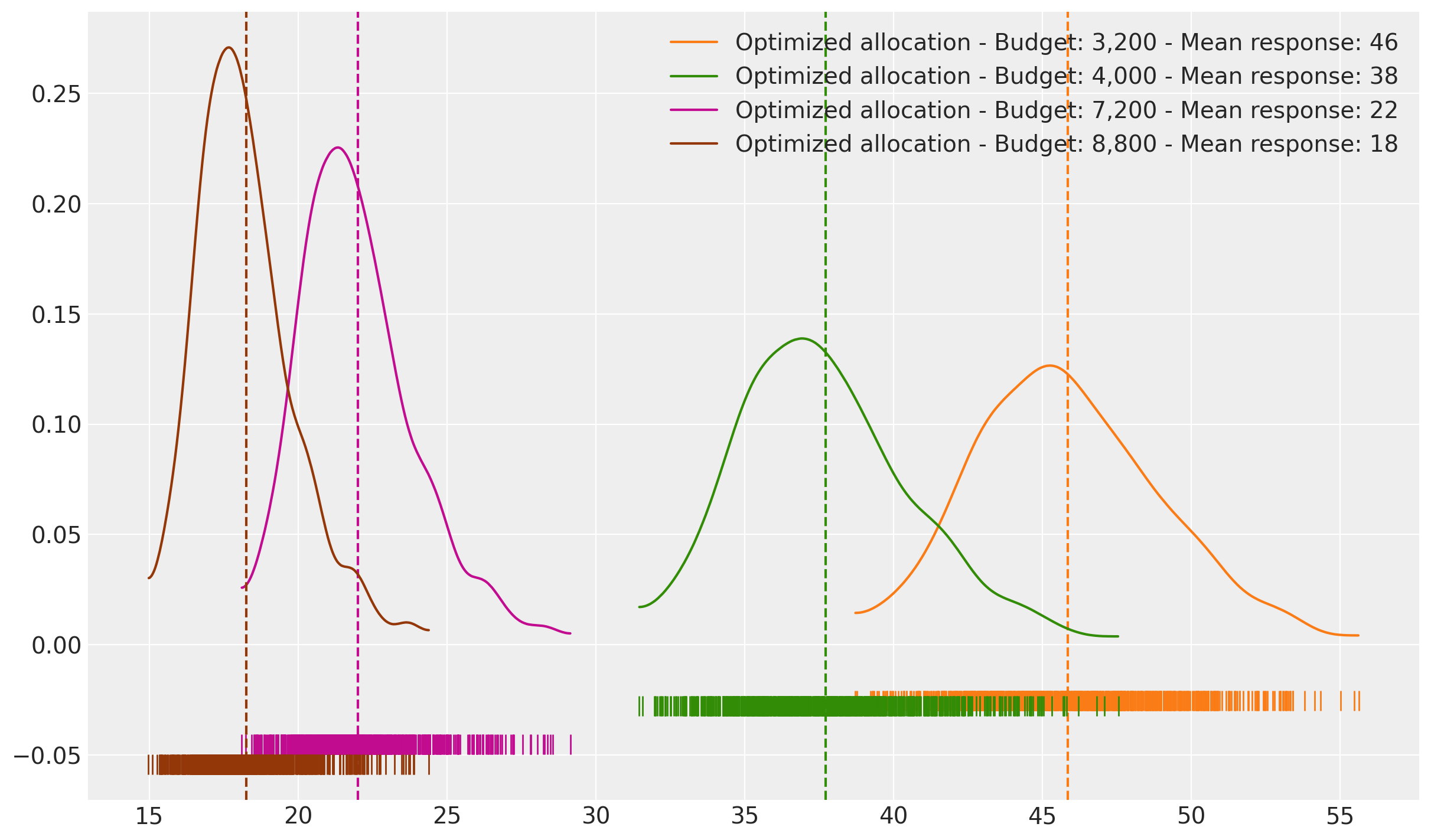
scenarios = np.array([0.8, 1, 1.8, 2.2])
colors = ["blue", "green", "red", "purple"]

# Create a larger figure with 2 rows
fig = plt.figure(figsize=(18, 22), layout="constrained")
gs = fig.add_gridspec(2, 1, height_ratios=[1, 1])

# Create a 2x2 grid for budget allocations in the top row
gs_top = gs[0].subgridspec(2, 2)

# Store responses and allocations for later use
responses = []
allocations = []

# Budget allocations in a 2x2 grid
for i, scenario in enumerate(scenarios):
    row, col = divmod(i, 2)  # Calculate row and column position in 2x2 grid

    tmp_budget = time_unit_budget * scenario
    print(f"Optimization for budget: {tmp_budget:.2f}M")
    tmp_allocation_strategy, tmp_optimization_result = (
        optimizable_model.optimize_budget(
            budget=tmp_budget,
        )
    )

    # Save allocation for later use
    allocations.append(tmp_allocation_strategy)

    tmp_response = optimizable_model.sample_response_distribution(
        allocation_strategy=tmp_allocation_strategy,
        include_carryover=True,
        include_last_observations=False,
    )
    # Save response for later use
    responses.append(tmp_response)

    # Add subplot for budget allocation in 2x2 grid
    ax = fig.add_subplot(gs_top[row, col])
    _, ax = optimizable_model.plot.budget_allocation(samples=tmp_response, ax=ax)
    ax.set_title(f"Budget: {tmp_budget:.0f}M")

# Second row: Response distributions (spanning the full width)
ax_dist = fig.add_subplot(gs[1])
for i, response in enumerate(responses):
    az.plot_dist(
        response.total_media_contribution_original_scale.values.flatten(),
        rug=True,
        color=colors[i],
        label=(
            f"Budget: {scenarios[i] * time_unit_budget:,.0f} - "
            f"Mean response: {response.total_media_contribution_original_scale.values.flatten().mean():,.0f}"
        ),
        ax=ax_dist,
    )

    # Add vertical line for mean
    mean_value = (
        response.total_media_contribution_original_scale.values.flatten().mean()
    )
    ax_dist.axvline(mean_value, color=colors[i], linestyle="--")

ax_dist.set_title("Response Distributions for Different Budget Scenarios")
ax_dist.set_xlabel("Response")
ax_dist.set_ylabel("Density")
ax_dist.legend()

fig.suptitle(
    "Budget Allocation and Response Distributions for Different Scenarios",
    fontsize=18,
    fontweight="bold",
);

Optimization for budget: 3200.00M

Sampling: [y]

Optimization for budget: 4000.00M

Sampling: [y]

Optimization for budget: 7200.00M

Sampling: [y]

Optimization for budget: 8800.00M

Sampling: [y]

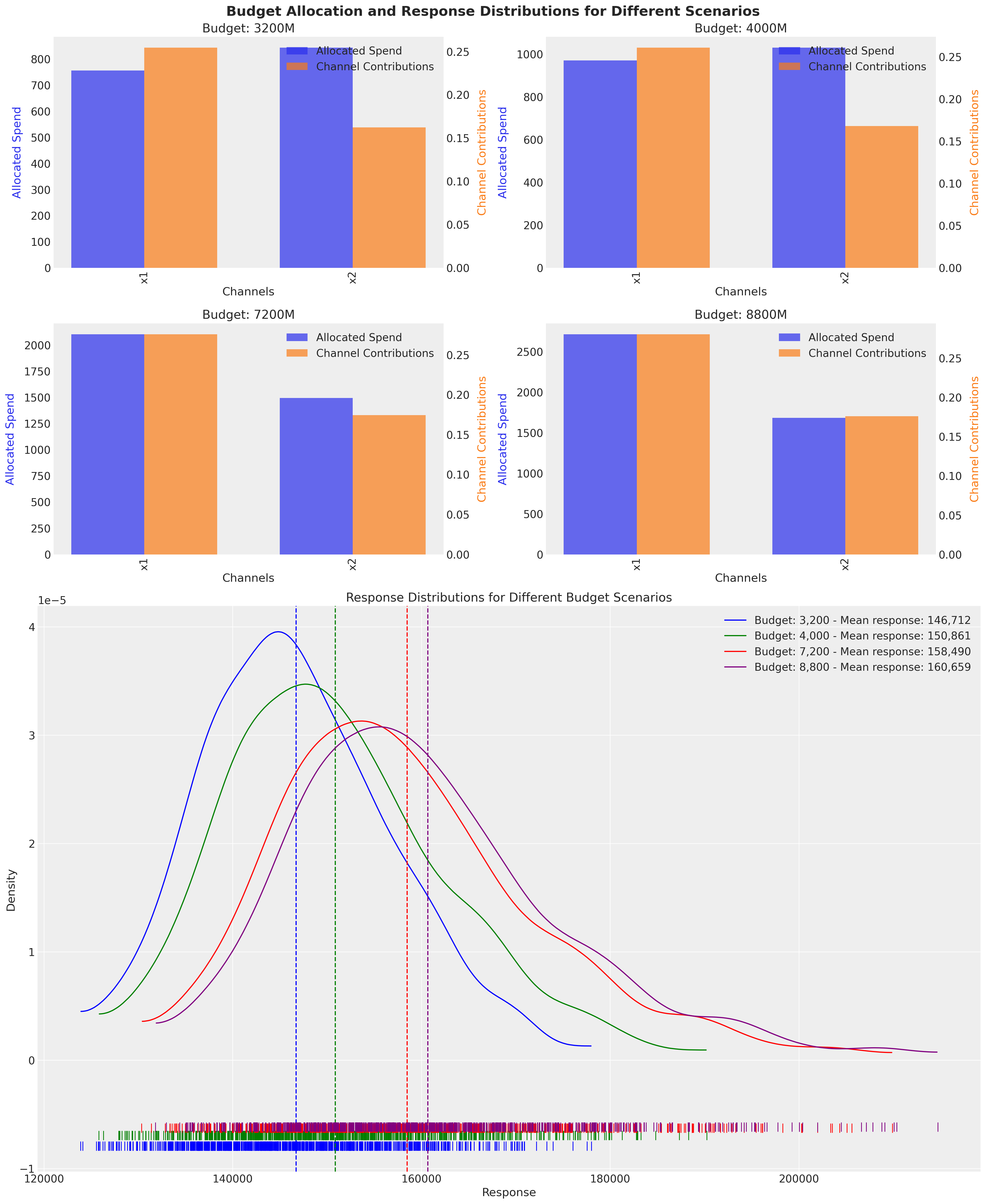
This makes everything clear, even adding the double of budget we can’t move our total response significantly. Of course, we are maximizing the response, but at what cost? Let’s take a look to the number of units back per unit spend, similar to ROAS.

fig, ax = plt.subplots()

for index, response in enumerate(responses):
    optimized_data = (
        response.total_media_contribution_original_scale.values.flatten()
        / allocations[index].sum().item()
    )
    optimized_mean = optimized_data.mean()
    az.plot_dist(
        optimized_data,
        # hdi_prob=0.75,
        color=f"C{index + 1}",
        label=(
            f"Optimized allocation - Budget: {scenarios[index] * time_unit_budget:,.0f} - "
            f"Mean response: {optimized_data.mean():,.0f}"
        ),
        ax=ax,
        rug=True,
        # kind="hist",
    )
    ax.axvline(optimized_mean, color=f"C{index + 1}", linestyle="--")

As expected, bigger the budget lower the returns. This happens because the response stays similar but the budget increases faster (Yes, the diminishing return effect). We can ask a different question, if we want to get 145,000, then what is the cheaper way to make it?

Optimizing towards a target

Another way to approach optimization is to adjust towards a target response. This can be useful if you want to ensure that the response is above a certain level. Instead of optimizing a given budget, we can optimize to find the right budget to reach a target response.

The following example shows how to create a custom constraint to minimize the budget to reach a target response. In short words, we are asking the optimizer, what is the minimum budget to reach a certain response?

import pytensor.tensor as pt

from pymc_marketing.mmm.budget_optimizer import BudgetOptimizer
from pymc_marketing.mmm.constraints import Constraint
from pymc_marketing.mmm.utility import _check_samples_dimensionality

target_response = 145_000


def mean_response_eq_constraint_fun(budgets_sym, total_budget_sym, optimizer):
    """Enforces mean_response(budgets_sym) = target_response, i.e. returns (mean_resp - target_response)."""
    resp_dist = optimizer.extract_response_distribution(
        "total_media_contribution_original_scale"
    )
    mean_resp = pt.mean(_check_samples_dimensionality(resp_dist))
    return mean_resp - target_response


def minimize_budget_utility(samples, budgets):
    return -pt.sum(budgets)


optimizer = BudgetOptimizer(
    num_periods=campaign_period,
    model=optimizable_model,
    response_variable="total_media_contribution_original_scale",
    utility_function=minimize_budget_utility,
    default_constraints=False,
    custom_constraints=[
        Constraint(
            key="target_response_constraint",
            constraint_fun=mean_response_eq_constraint_fun,
            constraint_type="ineq",
        )
    ],
)

allocation_xarray_target_response, res = optimizer.allocate_budget(
    total_budget=time_unit_budget // 2,
    x0=res_scipy.x,
    minimize_kwargs={"options": {"maxiter": 2_500}},
    budget_bounds=budget_bounds,
)

print("Optimal allocation:", allocation_xarray_target_response)
print("Solver result:", res)

Optimal allocation: <xarray.DataArray (geo: 2, channel: 2)> Size: 32B
array([[1527.44149652, 1282.08710607],
       [1548.87482853, 1289.99378633]])
Coordinates:
  * geo      (geo) <U5 40B 'geo_a' 'geo_b'
  * channel  (channel) <U2 16B 'x1' 'x2'
Solver result:      message: Optimization terminated successfully
     success: True
      status: 0
         fun: 5648.39721745586
           x: [ 1.527e+03  1.282e+03  1.549e+03  1.290e+03]
         nit: 26
         jac: [ 1.000e+00  1.000e+00  1.000e+00  1.000e+00]
        nfev: 27
        njev: 26
 multipliers: [ 4.636e-01]

sample_response_given_allocation_target_response = (
    optimizable_model.sample_response_distribution(
        allocation_strategy=allocation_xarray_target_response,
        include_carryover=True,
        include_last_observations=False,
    )
)

Sampling: [y]

sample_response_given_allocation_target_response

<xarray.Dataset> Size: 833kB
Dimensions:                                  (date: 21, geo: 2, sample: 800,
                                              channel: 2)
Coordinates:
  * date                                     (date) datetime64[ns] 168B 2021-...
  * geo                                      (geo) <U5 40B 'geo_a' 'geo_b'
  * channel                                  (channel) <U2 16B 'x1' 'x2'
  * sample                                   (sample) object 6kB MultiIndex
  * chain                                    (sample) int64 6kB 0 0 0 ... 1 1 1
  * draw                                     (sample) int64 6kB 0 1 ... 398 399
Data variables:
    y                                        (date, geo, sample) float64 269kB ...
    channel_contribution                     (date, geo, channel, sample) float64 538kB ...
    total_media_contribution_original_scale  (sample) float64 6kB 1.54e+05 .....
    allocation                               (geo, channel) float64 32B 1.527...
    x1                                       (date, geo) float64 336B 1.528e+...
    x2                                       (date, geo) float64 336B 1.281e+...
Attributes:
    created_at:                 2025-07-26T13:44:44.502389+00:00
    arviz_version:              0.22.0
    inference_library:          pymc
    inference_library_version:  5.25.1

xarray.Dataset

• Dimensions:
  • date: 21
  • geo: 2
  • sample: 800
  • channel: 2
• Coordinates: (6)
  • date
    (date)
    datetime64[ns]
    2021-09-06 ... 2022-01-24

    array(['2021-09-06T00:00:00.000000000', '2021-09-13T00:00:00.000000000',
           '2021-09-20T00:00:00.000000000', '2021-09-27T00:00:00.000000000',
           '2021-10-04T00:00:00.000000000', '2021-10-11T00:00:00.000000000',
           '2021-10-18T00:00:00.000000000', '2021-10-25T00:00:00.000000000',
           '2021-11-01T00:00:00.000000000', '2021-11-08T00:00:00.000000000',
           '2021-11-15T00:00:00.000000000', '2021-11-22T00:00:00.000000000',
           '2021-11-29T00:00:00.000000000', '2021-12-06T00:00:00.000000000',
           '2021-12-13T00:00:00.000000000', '2021-12-20T00:00:00.000000000',
           '2021-12-27T00:00:00.000000000', '2022-01-03T00:00:00.000000000',
           '2022-01-10T00:00:00.000000000', '2022-01-17T00:00:00.000000000',
           '2022-01-24T00:00:00.000000000'], dtype='datetime64[ns]')

  • geo
    (geo)
    <U5
    'geo_a' 'geo_b'

    array(['geo_a', 'geo_b'], dtype='<U5')

  • channel
    (channel)
    <U2
    'x1' 'x2'

    array(['x1', 'x2'], dtype='<U2')

  • sample
    (sample)
    object
    MultiIndex

    [800 values with dtype=object]

  • chain
    (sample)
    int64
    0 0 0 0 0 0 0 0 ... 1 1 1 1 1 1 1 1

    [800 values with dtype=int64]

  • draw
    (sample)
    int64
    0 1 2 3 4 5 ... 395 396 397 398 399

    [800 values with dtype=int64]

• Data variables: (6)
  • y
    (date, geo, sample)
    float64
    0.9543 0.9319 ... 0.4337 0.489

    array([[[0.95429769, 0.93189322, 0.98339488, ..., 1.12603735,
             1.04102115, 1.05599727],
            [1.06456706, 0.9688872 , 1.01717322, ..., 1.03790212,
             1.06019428, 1.02540066]],
    
           [[0.97137999, 0.98464263, 1.01103716, ..., 1.02410713,
             1.06931026, 1.07422391],
            [0.94979773, 0.8708559 , 0.96774448, ..., 1.12816251,
             1.098496  , 1.07578679]],
    
           [[1.03629215, 0.94834352, 0.98949923, ..., 1.06875629,
             1.10233011, 1.08046959],
            [1.0961887 , 1.01085747, 1.04408628, ..., 1.13008545,
             1.0738043 , 1.08848795]],
    
           ...,
    
           [[0.42108653, 0.60132672, 0.40262446, ..., 0.52169682,
             0.49438778, 0.70606934],
            [0.52466233, 0.49749332, 0.49197655, ..., 0.47918029,
             0.50826101, 0.50787444]],
    
           [[0.42144288, 0.58375695, 0.52379666, ..., 0.54667757,
             0.42837169, 0.67697119],
            [0.46688979, 0.4655064 , 0.45071721, ..., 0.46535356,
             0.43050558, 0.41706059]],
    
           [[0.39515945, 0.4600563 , 0.44046989, ..., 0.56530141,
             0.53984096, 0.48793108],
            [0.444341  , 0.44302096, 0.51894418, ..., 0.48468296,
             0.43373494, 0.48903367]]], shape=(21, 2, 800))

  • channel_contribution
    (date, geo, channel, sample)
    float64
    0.3884 0.3828 0.3563 ... 0.0 0.0

    array([[[[3.88399913e-01, 3.82830756e-01, 3.56260942e-01, ...,
              3.65496356e-01, 3.46195438e-01, 3.72107835e-01],
             [2.21045825e-01, 1.98383516e-01, 2.31795308e-01, ...,
              2.80718752e-01, 3.10978062e-01, 2.63104727e-01]],
    
            [[3.88444104e-01, 3.82891045e-01, 3.56292973e-01, ...,
              3.65614562e-01, 3.46214834e-01, 3.72198517e-01],
             [2.21048861e-01, 1.98386801e-01, 2.31804361e-01, ...,
              2.80880672e-01, 3.11432918e-01, 2.63243320e-01]]],
    
    
           [[[3.88814707e-01, 3.83404741e-01, 3.56549108e-01, ...,
              3.66731229e-01, 3.46356342e-01, 3.73042808e-01],
             [2.21074172e-01, 1.98414662e-01, 2.31895912e-01, ...,
              2.82910969e-01, 3.19797950e-01, 2.64982923e-01]],
    
            [[3.88817034e-01, 3.83410666e-01, 3.56551160e-01, ...,
              3.66747249e-01, 3.46358002e-01, 3.73050852e-01],
             [2.21075143e-01, 1.98415730e-01, 2.31898615e-01, ...,
              2.82989941e-01, 3.20019425e-01, 2.65048778e-01]]],
    ...
              1.34506887e-03, 7.58343551e-04, 3.37382455e-03],
             [4.45527071e-07, 4.18914855e-07, 1.86993124e-06, ...,
              1.44646472e-06, 1.95978785e-05, 1.51335230e-06]],
    
            [[5.57238233e-03, 1.61103709e-03, 2.56739239e-03, ...,
              1.36340244e-03, 7.68679991e-04, 3.41980834e-03],
             [4.48526373e-07, 4.21735002e-07, 1.88251967e-06, ...,
              1.45620236e-06, 1.97298120e-05, 1.52354023e-06]]],
    
    
           [[[0.00000000e+00, 0.00000000e+00, 0.00000000e+00, ...,
              0.00000000e+00, 0.00000000e+00, 0.00000000e+00],
             [0.00000000e+00, 0.00000000e+00, 0.00000000e+00, ...,
              0.00000000e+00, 0.00000000e+00, 0.00000000e+00]],
    
            [[0.00000000e+00, 0.00000000e+00, 0.00000000e+00, ...,
              0.00000000e+00, 0.00000000e+00, 0.00000000e+00],
             [0.00000000e+00, 0.00000000e+00, 0.00000000e+00, ...,
              0.00000000e+00, 0.00000000e+00, 0.00000000e+00]]]],
          shape=(21, 2, 2, 800))

  • total_media_contribution_original_scale
    (sample)
    float64
    1.54e+05 1.427e+05 ... 1.57e+05

    array([153971.79552486, 142726.1639974 , 145854.08393629, 155654.31243905,
           170257.44305342, 149143.52714982, 149014.69796627, 166053.23330852,
           185637.37235374, 150524.75250394, 151324.13553546, 164483.53039236,
           177852.62545105, 159110.28983548, 141361.82143607, 176769.23846053,
           176114.99238047, 141225.38276796, 143583.87505523, 145419.54041319,
           144030.47436191, 148151.09871268, 157251.28333534, 163507.00811574,
           164636.2508391 , 145695.56481969, 157967.58910367, 148571.47320362,
           170884.31749289, 173310.73824311, 149333.8865839 , 146571.23971738,
           153662.71790341, 152557.17672194, 166375.23026135, 161219.08028793,
           182199.26819425, 162493.34983316, 161116.38300112, 156693.2184675 ,
           142147.02926915, 138664.83434919, 168777.35394735, 144008.1799926 ,
           147005.39853408, 144166.33027915, 151719.81587273, 148770.13395656,
           154298.82295671, 162620.47389058, 150338.73026513, 153123.73550425,
           154212.47741068, 152250.68137735, 156607.25201036, 157919.83138455,
           173924.80693079, 160063.13851257, 182373.28292001, 168057.9456218 ,
           156170.96598792, 152207.30555027, 157958.37728264, 164068.6026339 ,
           162976.03680193, 177372.39096711, 182828.03368474, 146245.93410603,
           152139.57036677, 153672.32254353, 153971.79391603, 171030.79728934,
           153047.23106748, 140882.12252473, 133155.95972625, 144447.67242304,
           159298.67820474, 153653.68278278, 164154.27297344, 137438.10455242,
    ...
           149540.43092584, 169942.38907404, 150323.51553085, 154188.88034998,
           152617.13613014, 152090.59074928, 155102.08251735, 163201.26213489,
           144202.30704101, 163429.21732166, 156112.89197691, 165970.78222183,
           156180.72382192, 159476.00455183, 195651.66384665, 199076.50608296,
           146407.86338318, 148765.94789583, 152159.93985887, 137084.10432529,
           140144.9947824 , 161067.03367962, 147634.08953142, 148816.12551955,
           163567.40228021, 149339.63966785, 163361.27220975, 169862.56031245,
           152260.11009054, 176475.94580384, 175614.21221342, 160861.93923823,
           138436.52910093, 162744.45039229, 141333.85460757, 164633.06048908,
           147526.65952352, 144723.26245001, 146136.15584978, 164160.37183608,
           152975.38424596, 150296.83519469, 163677.23011017, 152124.82216264,
           147872.54561732, 176321.94136852, 147134.67527182, 143628.22176092,
           149684.56635236, 138652.59157881, 141266.63915547, 132254.05747988,
           133861.23367658, 143490.3466598 , 172016.50840241, 167450.69298535,
           163590.78825954, 146537.02430148, 164588.07234609, 158468.42390847,
           167706.88524392, 170132.44451017, 188428.61155507, 146951.93479188,
           148123.08979252, 179119.20044779, 172743.33400652, 146196.70892094,
           136576.883807  , 177208.73013809, 173970.78270911, 176290.49475795,
           147396.67937641, 155649.41298817, 149961.41920033, 151533.4831812 ,
           147742.70518315, 156344.99869126, 160251.56210916, 157037.86186676])

  • allocation
    (geo, channel)
    float64
    1.527e+03 1.282e+03 ... 1.29e+03

    array([[1527.44149652, 1282.08710607],
           [1548.87482853, 1289.99378633]])

  • x1
    (date, geo)
    float64
    1.528e+03 1.55e+03 ... 0.0 0.0

    array([[1527.91019959, 1550.02914117],
           [1524.44049582, 1549.07146729],
           [1527.41565369, 1550.22748171],
           [1527.54306218, 1549.59393184],
           [1528.00869355, 1550.22602403],
           [1527.15714897, 1550.75529047],
           [1526.78266059, 1549.69360425],
           [1528.07634456, 1552.16902127],
           [1526.65358619, 1549.82230231],
           [1527.26622731, 1547.60664602],
           [1528.58473899, 1547.85116934],
           [1527.62097775, 1550.21522382],
           [1528.48577296, 1549.3195399 ],
           [   0.        ,    0.        ],
           [   0.        ,    0.        ],
           [   0.        ,    0.        ],
           [   0.        ,    0.        ],
           [   0.        ,    0.        ],
           [   0.        ,    0.        ],
           [   0.        ,    0.        ],
           [   0.        ,    0.        ]])

  • x2
    (date, geo)
    float64
    1.281e+03 1.291e+03 ... 0.0 0.0

    array([[1280.74964444, 1291.2033906 ],
           [1280.41245055, 1289.58708557],
           [1280.99005708, 1290.99405822],
           [1283.53678385, 1288.88870147],
           [1280.85394426, 1289.92957959],
           [1281.21140313, 1289.79505517],
           [1281.63424808, 1290.46376218],
           [1282.6411593 , 1289.47112018],
           [1281.04056143, 1291.44569036],
           [1281.00663086, 1290.83047497],
           [1282.78562443, 1290.29235518],
           [1282.36834845, 1290.28133925],
           [1282.17401549, 1290.80564852],
           [   0.        ,    0.        ],
           [   0.        ,    0.        ],
           [   0.        ,    0.        ],
           [   0.        ,    0.        ],
           [   0.        ,    0.        ],
           [   0.        ,    0.        ],
           [   0.        ,    0.        ],
           [   0.        ,    0.        ]])

• Indexes: (4)
  • date
    PandasIndex

    PandasIndex(DatetimeIndex(['2021-09-06', '2021-09-13', '2021-09-20', '2021-09-27',
                   '2021-10-04', '2021-10-11', '2021-10-18', '2021-10-25',
                   '2021-11-01', '2021-11-08', '2021-11-15', '2021-11-22',
                   '2021-11-29', '2021-12-06', '2021-12-13', '2021-12-20',
                   '2021-12-27', '2022-01-03', '2022-01-10', '2022-01-17',
                   '2022-01-24'],
                  dtype='datetime64[ns]', name='date', freq=None))

  • geo
    PandasIndex

    PandasIndex(Index(['geo_a', 'geo_b'], dtype='object', name='geo'))

  • channel
    PandasIndex

    PandasIndex(Index(['x1', 'x2'], dtype='object', name='channel'))

  • sample
    chain
    draw
    PandasMultiIndex

    PandasIndex(MultiIndex([(0,   0),
                (0,   1),
                (0,   2),
                (0,   3),
                (0,   4),
                (0,   5),
                (0,   6),
                (0,   7),
                (0,   8),
                (0,   9),
                ...
                (1, 390),
                (1, 391),
                (1, 392),
                (1, 393),
                (1, 394),
                (1, 395),
                (1, 396),
                (1, 397),
                (1, 398),
                (1, 399)],
               name='sample', length=800))

• Attributes: (4)

  created_at :

  2025-07-26T13:44:44.502389+00:00

  arviz_version :

  0.22.0

  inference_library :

  pymc

  inference_library_version :

  5.25.1

fig, ax = plt.subplots()

# Initial planned allocation
initial_data = sample_response_give_initial_budget.total_media_contribution_original_scale.values.flatten()
initial_mean = initial_data.mean()
az.plot_dist(
    initial_data,
    # hdi_prob=0.75,
    color="blue",
    label=f"Intial planned allocation: Response {initial_mean:,.0f}",
    ax=ax,
    # kind="hist",
)
ax.axvline(initial_mean, color="blue", linestyle="--")

# Optimized allocation based on maximizing the response
optimized_data = sample_response_given_allocation.total_media_contribution_original_scale.values.flatten()
optimized_mean = optimized_data.mean()
az.plot_dist(
    optimized_data,
    # hdi_prob=0.75,
    color="red",
    label=f"Optimized allocation Maximizing: Response {optimized_mean:,.0f}",
    ax=ax,
    # kind="hist",
)
ax.axvline(optimized_mean, color="red", linestyle="--")

# Optimized allocation based on minimizing the budget
optimized_data_target_response = sample_response_given_allocation_target_response.total_media_contribution_original_scale.values.flatten()  # noqa: E501
optimized_mean_target_response = optimized_data_target_response.mean()
az.plot_dist(
    optimized_data_target_response,
    # hdi_prob=0.75,
    color="green",
    label=f"Optimized allocation Minimizing: Response {optimized_mean_target_response:,.0f}",
    ax=ax,
    # kind="hist",
)
ax.axvline(optimized_mean_target_response, color="green", linestyle="--")

ax.set_title("Comparison of Intial and Optimized allocation")
ax.set_xlabel("Response")
ax.set_ylabel("Density")
ax.legend()

plt.show()

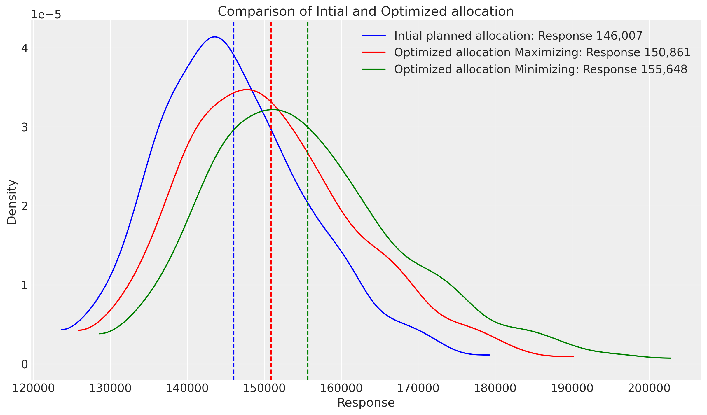
Great! Looks like using 5K euros, we could get a response even bigger than the initial optimization. Considering that the spend it’s slightly more in order to get this amount of response, ROAS should be good. Let’s take a look!

fig, ax = plt.subplots()

# Initial planned allocation
initial_data = (
    sample_response_give_initial_budget.total_media_contribution_original_scale.values.flatten()
    / initial_budget.sum().item()
)
initial_mean = initial_data.mean()
az.plot_dist(
    initial_data,
    # hdi_prob=0.75,
    color="blue",
    label=f"Intial planned allocation: Response {initial_mean:,.0f}",
    ax=ax,
    # kind="hist",
)
ax.axvline(initial_mean, color="blue", linestyle="--")

# Optimized allocation based on maximizing the response
optimized_data = (
    sample_response_given_allocation.total_media_contribution_original_scale.values.flatten()
    / allocation_xarray.sum().item()
)
optimized_mean = optimized_data.mean()
az.plot_dist(
    optimized_data,
    # hdi_prob=0.75,
    color="red",
    label=f"Optimized allocation Maximizing: Response {optimized_mean:,.0f}",
    ax=ax,
    # kind="hist",
)
ax.axvline(optimized_mean, color="red", linestyle="--")

# Optimized allocation based on minimizing the budget
optimized_data_target_response = (
    sample_response_given_allocation_target_response.total_media_contribution_original_scale.values.flatten()
    / allocation_xarray_target_response.sum().item()
)
optimized_mean_target_response = optimized_data_target_response.mean()
az.plot_dist(
    optimized_data_target_response,
    # hdi_prob=0.75,
    color="green",
    label=f"Optimized allocation Minimizing: Response {optimized_mean_target_response:,.0f}",
    ax=ax,
    # kind="hist",
)
ax.axvline(optimized_mean_target_response, color="green", linestyle="--")

ax.set_title("Comparison of Intial and Optimized allocation")
ax.set_xlabel("Response")
ax.set_ylabel("Density")
ax.legend()

plt.show()

The new result is much clearer. By using a bit more budget, we could achieve the more outcomes as our initial setup, in a more profitable way. On the other hand, the optimal allocation distributes the budget in levels similar by the model, not increasing the uncertainty around the estimated impact, at least not as much as going up a 2X more on budget.

Please note that the estimate provided assumes consistent spending each week. However, in the field of marketing, even with a fixed spending level, the actual spending can fluctuate based on factors such as the number of people bidding on your ad or viewing ads on a given day.

To account for this unpredictable variation, we have included a parameter called noise_level that allows you to introduce white noise into the projection. This can provide a sense of what the outcome might look like if the recommended budget could potentially fluctuate by a certain extent. The default value for noise_level is 1%, but you can adjust it as needed. In the example below, we have used a value of 10%.

Take a look to signature below!

optimizable_model.sample_response_distribution?

Signature:
optimizable_model.sample_response_distribution(
    allocation_strategy: 'xr.DataArray',
    noise_level: 'float' = 0.001,
    additional_var_names: 'list[str] | None' = None,
    include_last_observations: 'bool' = False,
    include_carryover: 'bool' = True,
    budget_distribution_over_period: 'xr.DataArray | None' = None,
) -> 'az.InferenceData'
Docstring:
Generate synthetic dataset and sample posterior predictive based on allocation.

Parameters
----------
allocation_strategy : DataArray
    The allocation strategy for the channels.
noise_level : float
    The relative level of noise to add to the data allocation.
additional_var_names : list[str] | None
    Additional variable names to include in the posterior predictive sampling.
include_last_observations : bool
    Whether to include the last observations for continuity.
include_carryover : bool
    Whether to include carryover effects.
budget_distribution_over_period : xr.DataArray | None
    Distribution factors for budget allocation over time. Should have dims ("date", *budget_dims)
    where date dimension has length num_periods. Values along date dimension should sum to 1 for
    each combination of other dimensions. If provided, multiplies the noise values by this distribution.

Returns
-------
az.InferenceData
    The posterior predictive samples based on the synthetic dataset.
File:      ~/Documents/GitHub/pymc-marketing/pymc_marketing/mmm/multidimensional.py
Type:      method

If you don’t want to assume a evenly distributed allocation given, you can use a custom pattern. Providing the optimizer a way around how to spend the money over time. The parameter it’s call budget_distribution_over_period and you can read about it in the following signature.

optimizer?

Type:           BudgetOptimizer
String form:    num_periods=12 mmm_model=<pymc_marketing.mmm.multidimensional.MultiDimensionalBudgetOptimizerWrap <...> Constraint object at 0x14f2ced80>] default_constraints=False budget_distribution_over_period=None
File:           ~/Documents/GitHub/pymc-marketing/pymc_marketing/mmm/budget_optimizer.py
Docstring:     
A class for optimizing budget allocation in a marketing mix model.

The goal of this optimization is to maximize the total expected response
by allocating the given budget across different marketing channels. The
optimization is performed using the Sequential Least Squares Quadratic
Programming (SLSQP) method, which is a gradient-based optimization algorithm
suitable for solving constrained optimization problems.

For more information on the SLSQP algorithm, refer to the documentation:
https://docs.scipy.org/doc/scipy/reference/generated/scipy.optimize.minimize.html

Parameters
----------
num_periods : int
    Number of time units at the desired time granularity to allocate budget for.
model : MMMModel
    The marketing mix model to optimize.
response_variable : str, optional
    The response variable to optimize. Default is "total_contribution".
utility_function : UtilityFunctionType, optional
    The utility function to maximize. Default is the mean of the response distribution.
budgets_to_optimize : xarray.DataArray, optional
    Mask defining a subset of budgets to optimize. Non-optimized budgets remain fixed at 0.
custom_constraints : Sequence[Constraint], optional
    Custom constraints for the optimizer.
default_constraints : bool, optional
    Whether to add a default sum constraint on the total budget. Default is True.
budget_distribution_over_period : xarray.DataArray, optional
    Distribution factors for budget allocation over time. Should have dims ("date", *budget_dims)
    where date dimension has length num_periods. Values along date dimension should sum to 1 for
    each combination of other dimensions. If None, budget is distributed evenly across periods.
Init docstring:
Create a new model by parsing and validating input data from keyword arguments.

Raises [`ValidationError`][pydantic_core.ValidationError] if the input data cannot be
validated to form a valid model.

`self` is explicitly positional-only to allow `self` as a field name.

# Get dimensions from the sample response
dates = sample_response_give_initial_budget.date.values[
    : -(optimizable_model.adstock.l_max)
]
geos = sample_response_give_initial_budget.geo.values
channels = ["x1", "x2"]
n_dates = len(dates)

print(f"Number of dates: {n_dates}")
print(f"Number of geos: {len(geos)}")
print(f"Number of channels: {len(channels)}")

# Create decreasing values for each date that sum to 1
decreasing_values = np.linspace(0.5, 0, n_dates)
# Normalize to make the sum equal to 1
decreasing_values = decreasing_values / decreasing_values.sum()

# Create the data array with the specified dimensions
data = np.zeros((len(dates), len(geos), len(channels)))
for i in range(len(geos)):
    for j in range(len(channels)):
        data[:, i, j] = decreasing_values

# Create xarray DataArray with proper dimensions
custom_budget_distribution = xr.DataArray(
    data,
    dims=["date", "geo", "channel"],
    coords={"date": dates, "geo": geos, "channel": channels},
)

Number of dates: 13
Number of geos: 2
Number of channels: 2

Note: When using a custom budget distribution over time, ensure that the values for each channel and geo sum to 1 across the time dimension. This is demonstrated in the example above where we create decreasing values that are normalized to sum to 1.

custom_budget_distribution.sum(dim="date")

<xarray.DataArray (geo: 2, channel: 2)> Size: 32B
array([[1., 1.],
       [1., 1.]])
Coordinates:
  * geo      (geo) <U5 40B 'geo_a' 'geo_b'
  * channel  (channel) <U2 16B 'x1' 'x2'

xarray.DataArray

• geo: 2
• channel: 2

• 1.0 1.0 1.0 1.0

  array([[1., 1.],
         [1., 1.]])

• Coordinates: (2)
  • geo
    (geo)
    <U5
    'geo_a' 'geo_b'

    array(['geo_a', 'geo_b'], dtype='<U5')

  • channel
    (channel)
    <U2
    'x1' 'x2'

    array(['x1', 'x2'], dtype='<U2')

• Indexes: (2)
  • geo
    PandasIndex

    PandasIndex(Index(['geo_a', 'geo_b'], dtype='object', name='geo'))

  • channel
    PandasIndex

    PandasIndex(Index(['x1', 'x2'], dtype='object', name='channel'))

• Attributes: (0)

We can pass this new parameter in the optimizable model.

allocation_xarray_custom_budget_distribution, _ = optimizable_model.optimize_budget(
    budget=time_unit_budget,  # Total budget to allocate here
    budget_distribution_over_period=custom_budget_distribution,
    minimize_kwargs={"options": {"maxiter": 2_000}},
    budget_bounds=budget_bounds,
)

sample_response_given_allocation_custom_budget_distribution = (
    optimizable_model.sample_response_distribution(
        allocation_strategy=allocation_xarray_custom_budget_distribution,
        include_carryover=True,
        include_last_observations=False,
        budget_distribution_over_period=custom_budget_distribution,
    )
)

Sampling: [y]

You can visualize the pattern for your variables access to the response sample!

sample_response_given_allocation_custom_budget_distribution["x1"].plot(hue="geo");

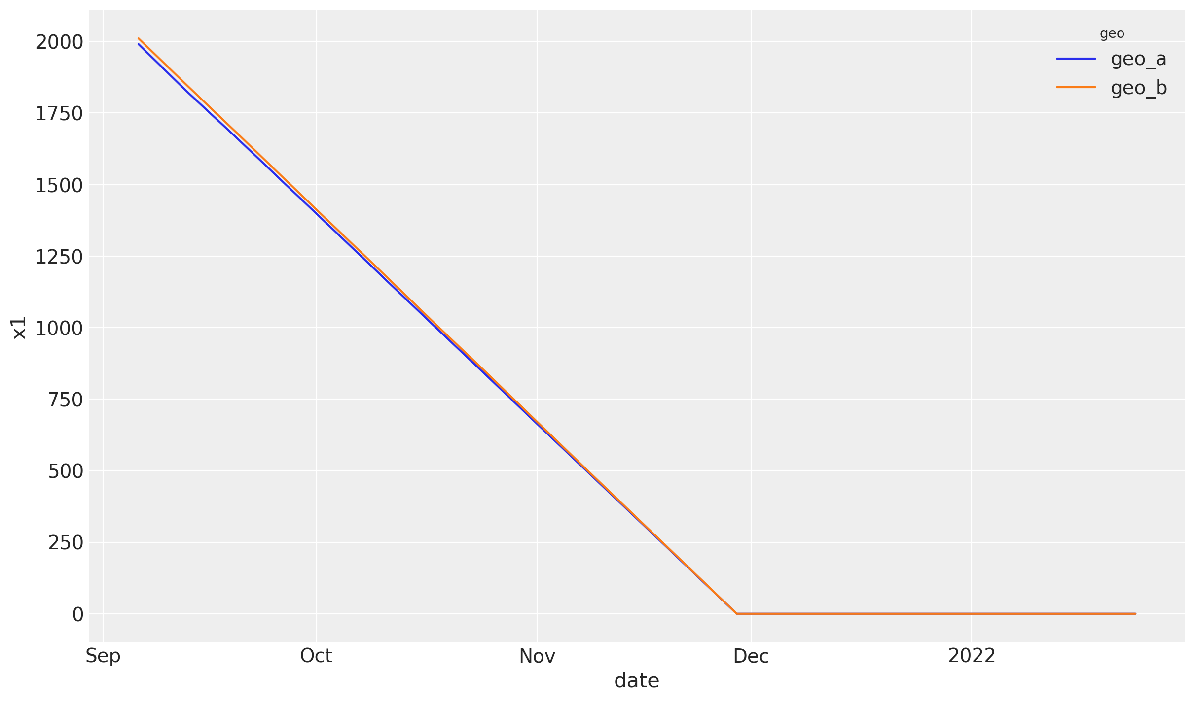
And giving that pattern, you’ll see some response!

optimizable_model.plot.allocated_contribution_by_channel_over_time(
    samples=sample_response_given_allocation_custom_budget_distribution,
);

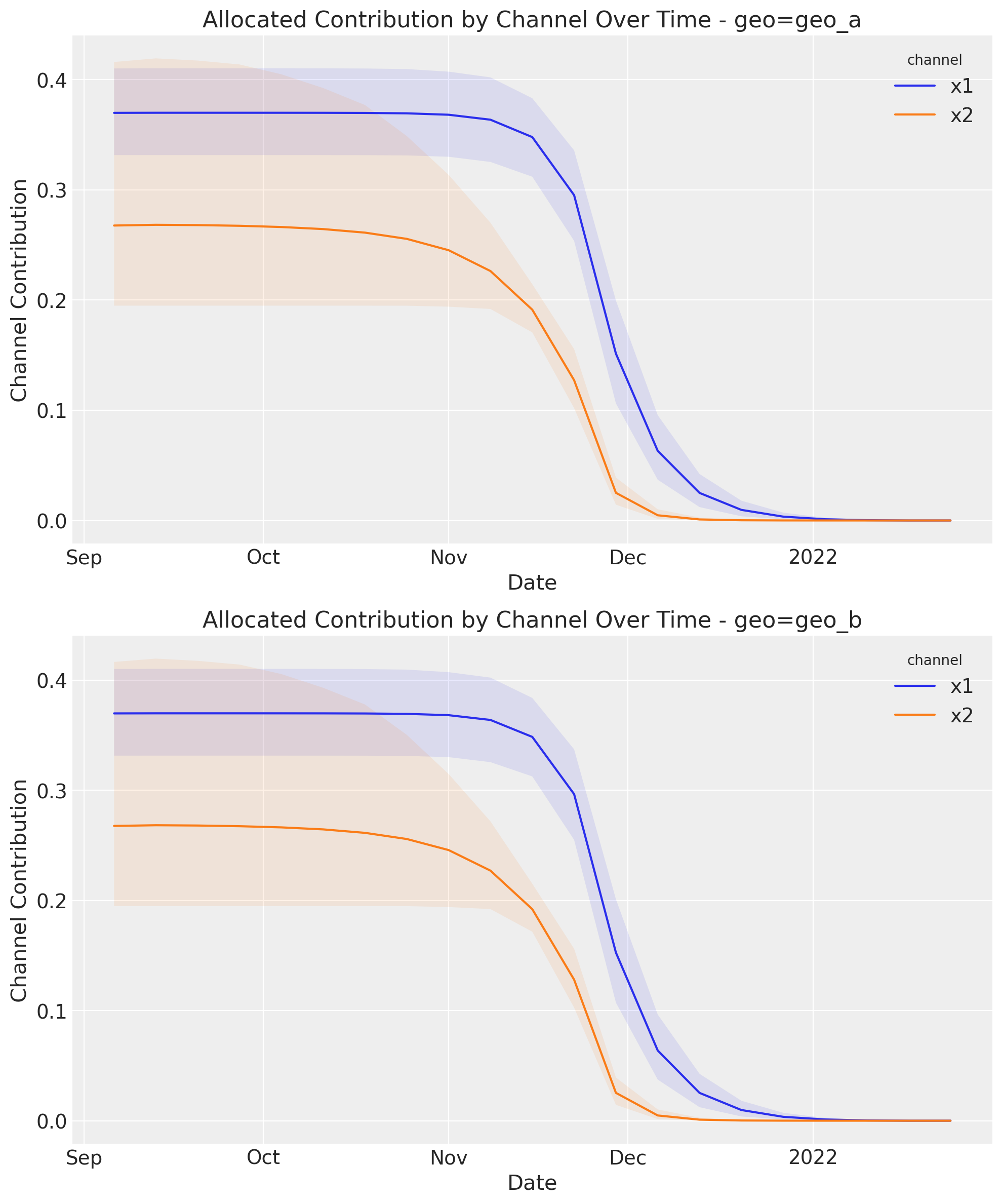
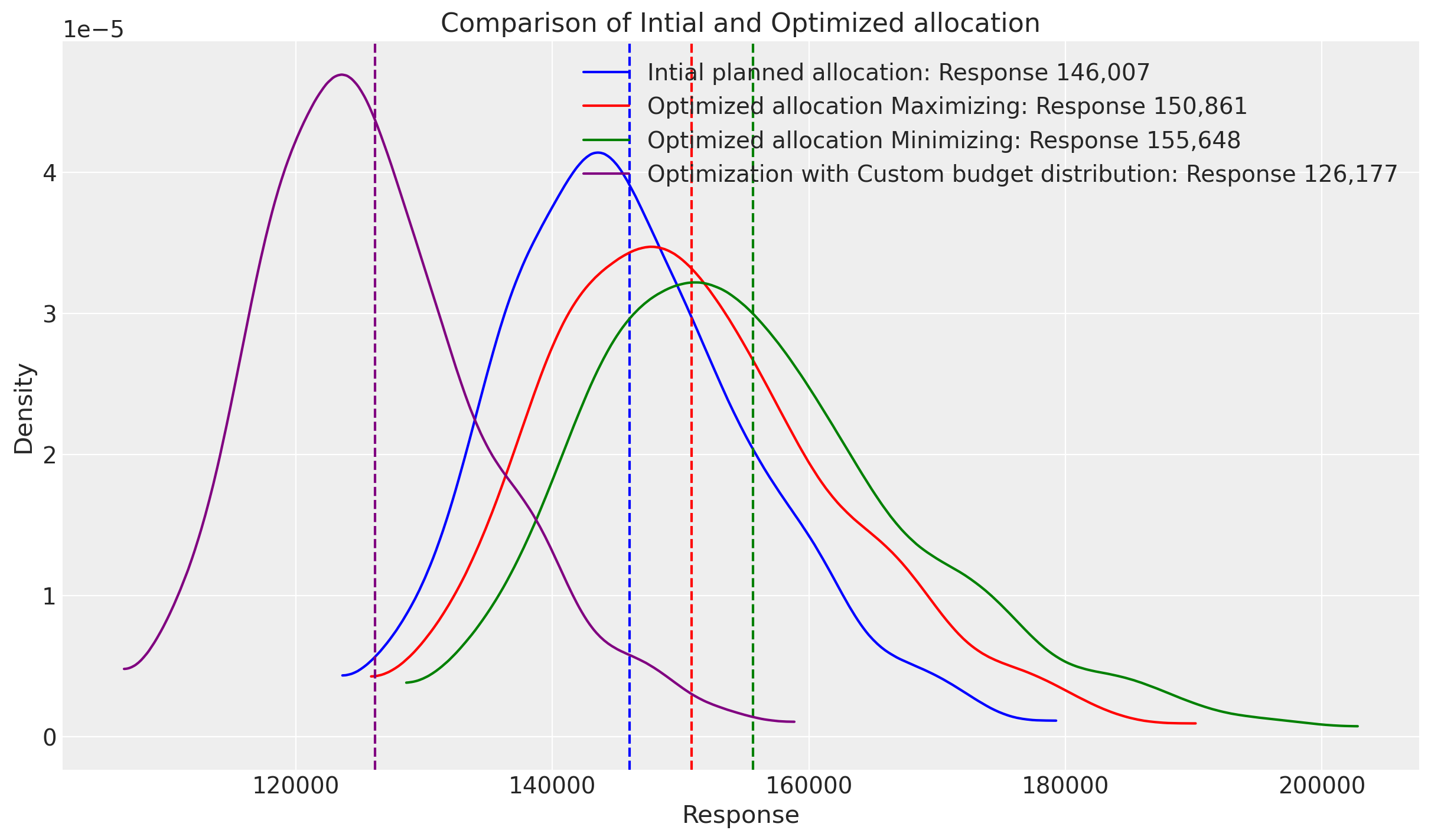
As expected, now the spend follows a specific pattern of spend, and the optimization process considers this as well. This change, can affect quite radically the total response, adding more or less complexity to your optimization challenges.

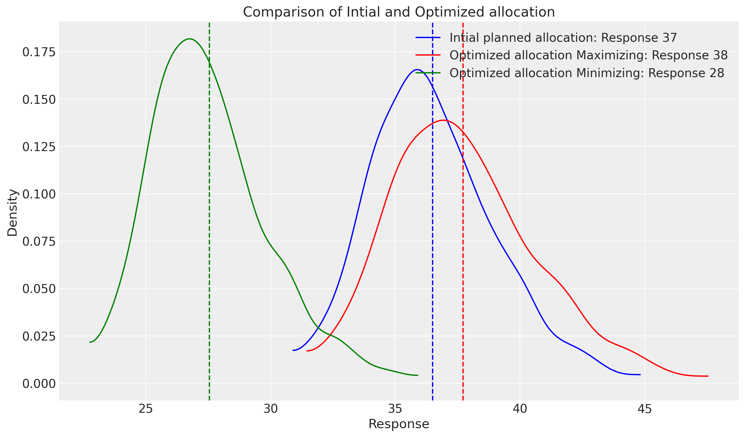
fig, ax = plt.subplots()

# Initial planned allocation
initial_data = sample_response_give_initial_budget.total_media_contribution_original_scale.values.flatten()
initial_mean = initial_data.mean()
az.plot_dist(
    initial_data,
    # hdi_prob=0.75,
    color="blue",
    label=f"Intial planned allocation: Response {initial_mean:,.0f}",
    ax=ax,
    # kind="hist",
)
ax.axvline(initial_mean, color="blue", linestyle="--")

# Optimized allocation based on maximizing the response
optimized_data = sample_response_given_allocation.total_media_contribution_original_scale.values.flatten()
optimized_mean = optimized_data.mean()
az.plot_dist(
    optimized_data,
    # hdi_prob=0.75,
    color="red",
    label=f"Optimized allocation Maximizing: Response {optimized_mean:,.0f}",
    ax=ax,
    # kind="hist",
)
ax.axvline(optimized_mean, color="red", linestyle="--")

# Optimized allocation based on minimizing the budget
optimized_data_target_response = sample_response_given_allocation_target_response.total_media_contribution_original_scale.values.flatten()  # noqa: E501
optimized_mean_target_response = optimized_data_target_response.mean()
az.plot_dist(
    optimized_data_target_response,
    # hdi_prob=0.75,
    color="green",
    label=f"Optimized allocation Minimizing: Response {optimized_mean_target_response:,.0f}",
    ax=ax,
    # kind="hist",
)
ax.axvline(optimized_mean_target_response, color="green", linestyle="--")

ax.set_title("Comparison of Intial and Optimized allocation")
ax.set_xlabel("Response")
ax.set_ylabel("Density")
ax.legend()

# Optimized allocation maximizing response based on custom budget distribution
optimized_data_custom_budget_distribution = sample_response_given_allocation_custom_budget_distribution.total_media_contribution_original_scale.values.flatten()  # noqa: E501
optimized_mean_custom_budget_distribution = (
    optimized_data_custom_budget_distribution.mean()
)
az.plot_dist(
    optimized_data_custom_budget_distribution,
    color="purple",
    label=f"Optimization with Custom budget distribution: Response {optimized_mean_custom_budget_distribution:,.0f}",
    ax=ax,
)
ax.axvline(optimized_mean_custom_budget_distribution, color="purple", linestyle="--")

ax.set_title("Comparison of Intial and Optimized allocation")
ax.set_xlabel("Response")
ax.set_ylabel("Density")
ax.legend()

plt.show()

Other methods to explore

The current optimization use the full posterior, and it can be use for more than minimize or maximize, can consider all information to perfom risk assesments, you can take a read to Risk Allocation for Media Mix Models. At the same time, it could be a powerful and interesting solution as it’s described on the following blog “Using bayesian decision making to optimize supply chains”

The current methodology is similar to the ones used on other libraries as Robyn from Meta and Google Lightweight from Google. You can explore the solutions and compare if needed.

Conclusion

MMM models and methodologies used here are designed to bridge the gap between theoretical rigor and actionable marketing insights. They represent a significant stride towards a more data-driven, analytical approach to marketing budget allocation, which could change how organizations invest in customer acquisition and retention.

Consequently, your engagements, feedback, and thoughts are not merely welcomed but actively solicited to make this tool as practical and universally applicable as possible.

%load_ext watermark
%watermark -n -u -v -iv -w -p pytensor

Last updated: Sat Jul 26 2025

Python implementation: CPython
Python version       : 3.12.11
IPython version      : 9.4.0

pytensor: 2.31.7

matplotlib    : 3.10.3
xarray        : 2025.7.1
pandas        : 2.3.1
pytensor      : 2.31.7
pymc_marketing: 0.15.1
numpy         : 2.2.6
arviz         : 0.22.0

Watermark: 2.5.0